
When considering integrating a photovoltaic installation into an existing or yet to be constructed building, all limitations must first be carefully studied.
Factors that influence the capacity (and therefore the profitability) of a system are:
1. the global solar radiation per year, expressed in kWh/m² / year
2. the orientation angle towards the south, expressed in degrees (°) (for a sloping roof or a facade)
3. the degree of inclination relative to a horizontal plane, expressed in degrees (°) (for a sloping roof)
4. the available surface area, expressed in m²
5. the technology used (efficiency expressed in Wp/m²)
6. 6. the method of integration or installation
7. the shadow of objects (chimneys, roof structures)
Illustration 1 shows the distribution for Belgium of solar radiation on an ideally located surface and the electricity production that could be generated by a solar system that is optimally oriented (azimuth of 0° to the full south and an inclination of 35°).
The production figures in kWh/m² a year are based on a 1 kWp system with an efficiency (Performance Ratio - PR) of 75%.
This performance ratio is defined as the ratio of the final output to the reference output; it quantifies the efficiency of the system from the photovoltaic conversion in the solar panels (at a nominal peak power) to the actual output of the inverter(s).
The ratio is also the ratio of the amount of energy actually generated to the amount of energy that could have been generated in an ideal photovoltaic system without losses, at a temperature of 25° and uniform solar radiation.
The established value for Brussels is - 840 kWh/kWp for a PR of 75% - on the low side; in general, 850 kWh/kWp is used for projects in Brussels.
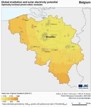
Illustration 1
Illustration 1: Solar map of Belgium with global solar radiation in kWh/m² a year and electricity production in kWh for an ideally oriented system (south, 35° tilt) with an efficiency of 75% (PVGIS © European Communities, 2001-2008)
The location of the installation on the roof is crucial. Ideally, an installation (at our latitude) is oriented directly to the south with an angle of inclination of 35°. However, a system that is positioned between west and east still provides sufficient yield at an angle of inclination between 20° and 60°. A deviation from the ideal position therefore only results in a loss of yield of a few percent (see Illustration below).
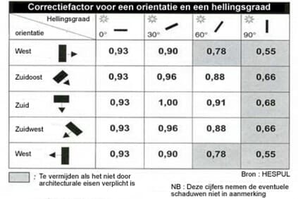
Illustration 2
Illustration 2: Correction factor (CF) for calculating the efficiency of a photovoltaic installation
The solar disk of Illustration 3 is a graphic representation of the loss of efficiency: this is the global solar radiation in Uccle as a function of the orientation and the inclination of the inclined plane. The correction factor (CF) is also expressed here in % and goes from yellow (100%) to blue (30%). (Note: Uccle is the largest municipality in terms of surface area in the Brussels-Capital Region after the city of Brussels and is located south of the centre of Brussels.)
It will be noted that there is a rather important zone for which the orientation and the angle of inclination do not have much influence on the solar radiation: namely the zone going from west/southwest to east/southeast, with an angle of inclination between 10° and 55°. The energy loss is less than 10% per year. The reason for this is the large share of scattered radiation at our latitude: in Belgium, approximately 60% of the solar energy reaches us in the form of scattered radiation.
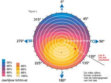
Illustration 3
Illustration 3: Annual relative radiation in Uccle on an inclined plane as a function of orientation (polar coordinates) and slope (radial coordinates)
Outside this optimal zone, for example, it has been found that the annual radiation loss of a vertical facade facing south is 27%, while for a horizontal surface it is only 13%.
Horizontal mounting of solar panels is generally not recommended, because dirt can easily accumulate. At least a 5° angle is required to allow the self-cleaning effect of rain to do its work.
The following conversion formula calculates the total production of the system (without shadow impact):
Production = Power (Wp) x Specific production of the installation x Correction factor [kWp x kWh/kWp x % = kWh/year]
Example: a 2.6 kWp system is on a roof with a slope of 50° and oriented to 120° east. From the solar disk we derive the correction factor: 85 %. The minimum production that must be achieved is:
2.6 x 850 x 0.85 = 1878.5 kWh/year.
The European Commission's Joint Research Centre website allows calculating the average system output based on input data for power, orientation, slope, physical location and technology. The site can be found at: Photovoltaic Geographical Information System (PVGIS). Available in English, French, Italian, Spanish and German.
Usually a flat rate system loss of 14% is taken into account, but this can be reduced to 12% through careful planning.
The available surface area and the method of integration determine the maximum capacity.
In the case of pitched roofs, the useful surface is delimited by the part facing south and not shaded by chimneys or other obstacles. In complex situations, an accurate inventory of all natural obstacles is always required, so that the impact of the shadow can be quantified. How the useful surface will translate into production capacity will depend on the efficiency of the chosen technology.
In the Brussels Region, green certificates are awarded based on the amount of energy produced and the size of the system in m². In this way, the technologies with the highest efficiency are favoured (modules with an efficiency of 17 to 18%), because they develop more power per m².
Eaves and cornices of flat roofs that receive a lot of radiation often reduce the useful surface area by 10 to 15%. This useful surface area can be exploited with horizontal amorphous modules or with modules in a sawtooth arrangement (sheds) (see page 6). In both cases, the peak capacity is approximately 60 to 70 Wp/m² roof surface.
Technology:
1. Crystalline technology, in sawtooth arrangement
Yield 1. 14 %
Surface area of the panels: 85 m², the maximum shadow angle between the rows is 17° and the angle of inclination is 35°
Peak power 11 kWp
2. Amorphous technology, horizontal (thin film technology)
Yield 2. 7 %
Surface area of the panels: 170 m²
Peak power 11 kWp
Example: A flat roof of 200 m² gross. This means approximately 170 m² of usable surface area if we take into account the eaves and cornices. With both technologies, the same peak power can be achieved on this surface area.
When a photovoltaic installation is integrated into a building (which is almost always the case in the Brussels Region), it is usually placed on the roof. In module 6 (Different types of installations) we look at the different ways in which this can be done: on flat and sloping roofs or integrated into the facade.
Photovoltaic installations that are shaded – even partially or temporarily – produce less energy on an annual basis.
In the Brussels-Capital Region, the energy premium for photovoltaic panels depended (among other things) on the professional preliminary study, which on the one hand maps out all natural obstacles that could cast shadows and on the other hand simulates the immediate environment on 21 December.
For obstacles that are far away from the solar panels (hills, cliffs), it is assumed that the radiation loss is evenly distributed over all panels (this depends on the size of the installation and the distance to the obstacle).
This does not apply to obstacles in the vicinity. The shadow that falls on one of the panels of a photovoltaic system can cause a significant loss in the entire installation. It is therefore important to take into account every possible shadow when estimating the annual production, even that resulting from relatively small obstacles (chimney, mast, antenna, ventilation pipes, etc.).
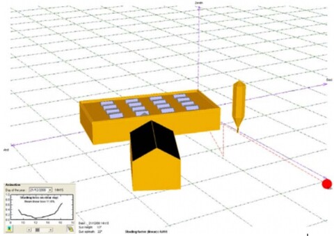
Illustration 4a
Illustration 4a is an example of a computer model for a photovoltaic installation on a flat roof with an 80 cm cornice and the shadow of a tree and a nearby building.
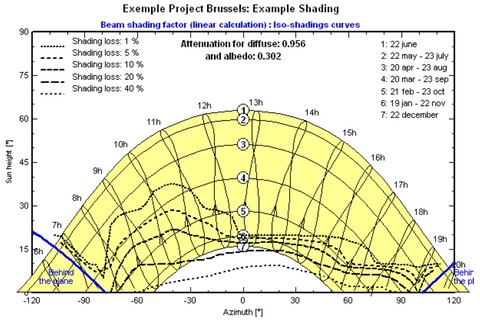
Illustration 4b
The yellow zone in Illustration 4b is a representation of the path of the sun for seven different periods of the year (the explanation can be found at the top right of the diagram), during an average day between 6:00 and 20:00. The dotted lines (the explanation can be found at the top left of the diagram) indicate the losses due to shadow. For the period from April 20 to August 23 (trajectory 3), there is 1% loss due to shadow between 7:00 and 13:00; the same is true for trajectory 4 from March 20 to September 23. Between trajectories 4 and 5, the losses increase to 5% for approximately the same time interval. And so on.
The project designer must evaluate the impact of shadow in the context of the installation and the performance ratio and, based on this, assess the viability of the photovoltaic project.
Example:
An installation of 3 kWp based on 2 levels of 8 modules of 185 Wp with electricity and a power supply of 2 100 W.
The shadow of a chimney falls on one of the fields. This causes a production reduction of approximately 1.5 kWh per day, or a total loss of +-10%.
Specialised software applications, such as PVSYST 2 (from the University of Geneva) or PVSOL 3, make it possible to model the building and its surroundings in a computer model and calculate the impact of shadow on this basis. These programmes take into account the position of the sun as a function of the latitude and longitude of the physical location of the installation. Since the position of the sun is known for every moment of the year, the software can calculate the impact of shadow. This method can be used for new and existing buildings and makes it possible to quantify the loss due to shadow. The detailed final report provides an overview of all losses – including shadow losses – expressed as a %.
The impact of shadow is a crucial issue, given the non-linear nature of the relationship between shadow and production loss. For the same percentage of shadow on a module, the impact can range from 0 to 100%, depending on the location of the shadow and the switching of the cells in the module.
Because the cells are connected in series, the cell that receives the least solar radiation (the one in the shade) determines how much current flows through the other cells. This is the so-called “garden hose effect”. If you squeeze a garden hose halfway, only half as much water comes out! If a solar cell is shaded by 50%, the PV production also drops by 50%. This negative effect can be limited by protections (bypass diodes) and so-called multi-string inverters.
Most panels are therefore equipped with bypass diodes, which limit the impact of shadow (and protect the cells). Nevertheless, the impact of shadow should not be underestimated.
From the beginning of the project, the impact of shadow formation must be studied in great detail. The installer must come on site and give his advice on all obstacles that can cause shadow. The financial and energy profitability of the project may depend on it.
If it is impossible to eliminate shadows, one can consider using certain technologies, such as amorphous aSi modules or hybrid (mixed amorphous and monocrystalline) HIT modules, as they are less susceptible to this problem.
Reading material: PVsyst
Reading material: Simulation software for renewable energy
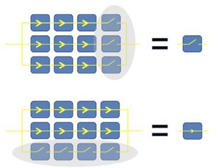
Illustration 5
Illustration 5: Comparison of the impact of shading on a photovoltaic panel in a cross-section and a longitudinal section and the (simplified) equivalent diagram.
In figures 6 and 7 we see an example of a panel with a portrait orientation in different shadow situations. The varying production losses can be explained by the presence of bypass diodes, which protect the panels from the harmful effects of shadow and which allow the shadowed panel and the other panels in the string to continue to function normally.
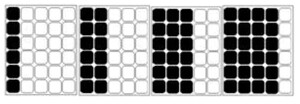
Illustration 6
Illustration 6: Four situations where the shadow covers vertical bands, causing a production loss of 30% to 100% (depending on the number of bypass diodes and the size of the shadowed part)
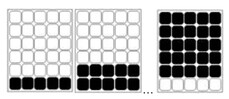
Illustration 7
Illustration 7: Three situations where the shadow covers horizontal bands (due to a poorly dimensioned sawtooth arrangement), causing a production loss of up to 100%.
Illustration 8
Illustration 8: Example of a shadow that causes almost 100% loss of production.
The maximum shadow angle technique is often used to anticipate the impact of shadow. In Belgium, this angle is 17°, but it can vary from 15° to 18.5°. The example of Illustration 9 shows that by respecting the maximum shadow angle of 17°, there is no shadow at 12 noon on 21 December. It should be noted that shadow has a very limited impact on global production in winter, since the winter months from November to February (one third of the year) contribute less than 1/6 of the annual production. Furthermore, shadow only hinders direct radiation, which during the period in question only accounts for about 30% of the solar energy; the rest is scattered radiation. However, shadow has a very pronounced impact during the months of April to September.
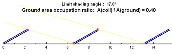
Illustration 9
Illustration 9: Influence of the inclination of the photovoltaic panels on the production losses, comparison of a sawtooth arrangement (sheds) with a single panel system (PVSYST software).
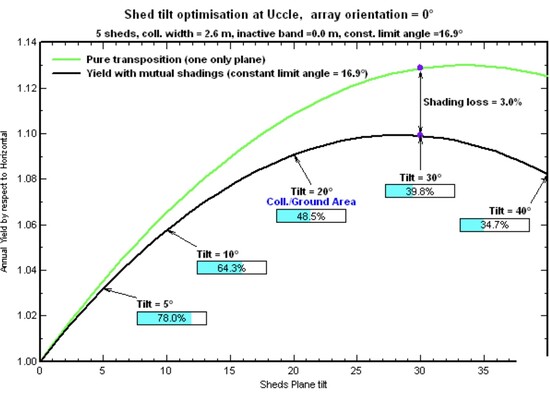
Illustration 10
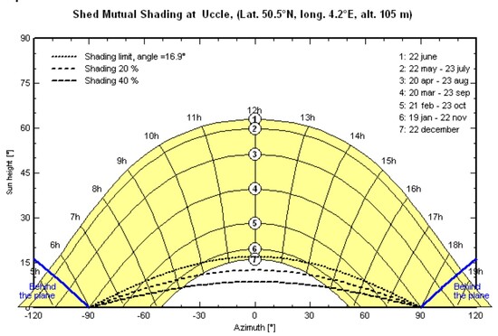
Illustration 11
The upper graph of Illustration 10 shows a comparison (green and black lines) between a single panel system and a system with multiple rows of panels, and the corresponding shading losses. In the case of multiple rows of panels (black line), the annual production increases with increasing slope and the available area decreases with increasing slope.
There are tools to visualize obstacles using optical techniques. A panoramic photo can already give an idea of the seriousness of the shadow problem at the project location (provided that there is a known reference point on the photo against which the angles of azimuth and slope can be calibrated).
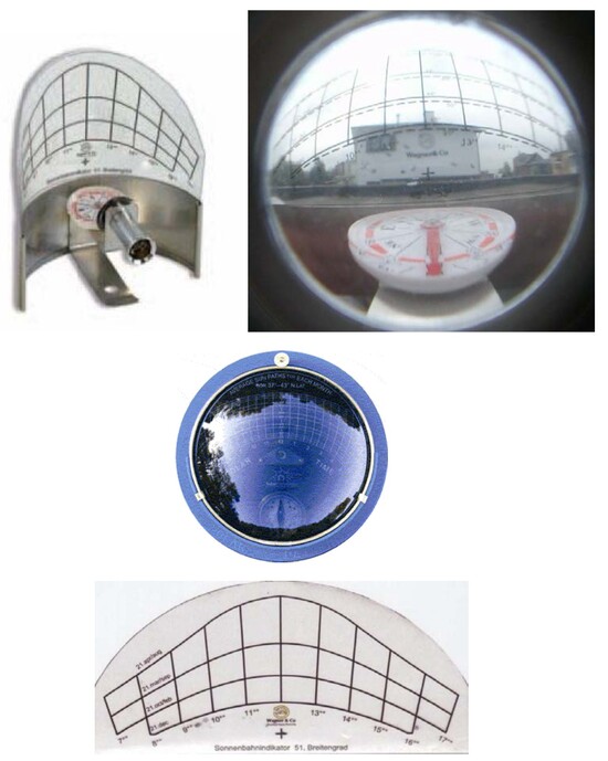
Illustration 12
Illustration 12: Example of an optical instrument used to visualize obstacles (shadow sources).
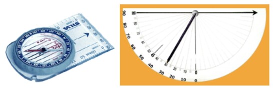
Illustration 13
Illustration 13: Other simple tools to visualize obstacles: compass and inclinometer
We can map the path of the shadow sources by connecting all the points of the azimuth/elevation combination. This curve can be limited to the most important shadow sources and therefore does not need to be drawn in great detail.
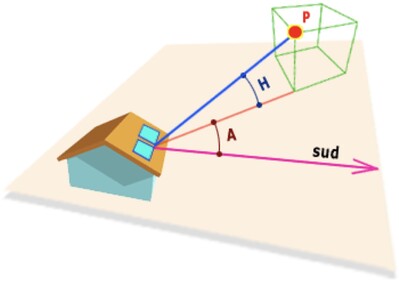
Illustration 14
Illustration 14: Azimuth - altitude
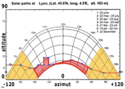
Illustration 15
Illustration 15: Shadow sources
In Illustration 15 the azimuth is on the x-axis, expressed as an angle with a value between –120° and +120°. In practice, azimuth values between -90° and +90° are sufficient. The elevation is on the y-axis, expressed as an angle with a value between 0° and 90°.
The beginning and end of the day [yellow areas in Illustration 15] have little influence and are therefore not taken into account. The total shadow of the obstacle is represented by the red area. In this way, the damage factor can be calculated, which must be applied when calculating the photovoltaic production of the field.
The calculation of this factor is very complex. It is based on geometric principles connected with shadow surfaces, the hour and calendar periods. Usually a special software is needed to calculate the factor precisely (for example PVSyst software).
If it turns out that shade is a significant problem at the project site, consideration may be given to relocating the panels, reducing their size, or changing their orientation.
For example, if it turns out that the shadows are becoming a problem during the afternoon, one could consider orienting the panels more to the east to capture more morning sun. An optimization often has to be carried out knowing that the geometry (orientation, angle of inclination and distance between the successive rows of panels) influences the production and therefore the financial return, with which the installation will ultimately pay for itself.